Conditional formatting is an Excel feature that allows users to customize the formatting of a single cell or group of cells based on whether a certain rule is satisfied. This feature is extremely useful in terms of automation, because the formatting of the selected cells changes automatically if the chosen condition is no longer satisfied (or becomes satisfied where it wasn’t satisfied before); otherwise, you would have to change the formatting by hand each time the condition is affected. For example, you may want to highlight cells with positive values green and cells with negative values red. If you use conditional formatting to do this, the highlight color automatically changes from green to red if a positive value then becomes negative, and vice versa:
Figure 1
There are seemingly countless options to choose from when setting up your conditional formatting; you aren’t just limited to the basic type of formatting shown in this brief example. This blog post provides an overview of the many, many different possibilities that exist within Excel’s conditional formatting module.
Accessing The Conditional Formatting Options
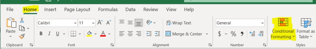
To access the conditional formatting menu, go to Home on the Excel ribbon, and then click on Conditional Formatting:
Figure 2
By doing so, the eight basic categories of options for conditional formatting appear: Highlight Cells Rules, Top/Bottom Rules, Data Bars, Color Scales, Icon Sets, New Rule, Clear Rules, and Manage Rules. As you’ll see, there’s a lot of overlap in terms of the capabilities offered by each option; in most circumstances, there’s more than one way of doing things with conditional formatting. Let’s dive into an in-depth review of each of those options. If you want to follow along, download an Excel version of UCI’s Auto-mpg dataset ―which is the dataset I’m using― from the UCI website or from Kaggle.
Highlight Cells Rules
Highlight Cells Rules has seven sub-options: Greater Than, Less Than, Between, Equal To, Text that Contains, A Date Occurring, and Duplicate Values (there’s also the More Rules button, but that brings up the same screen as the New Rule option which we’ll explore later).
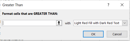
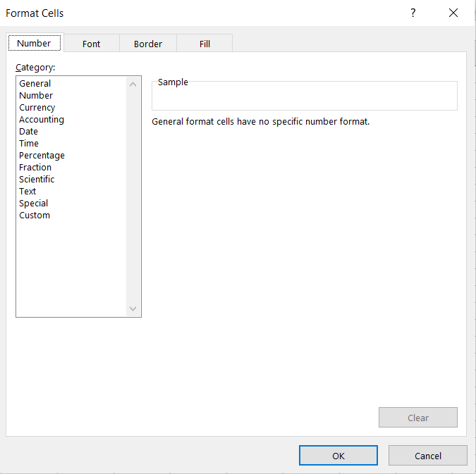
Greater Than. This sub-option allows you to highlight in a customizable way cell(s) that contain values greater than some other value. The value that you’re comparing to can either be a hard-coded value (such as simply “9”) or the value in another cell accessed via a cell reference (when in doubt, it’s always better to cell reference than to hardcode because cell referencing will allow the conditional formatting to update itself automatically when the value in the cell you’re referencing changes). When clicking on Greater Than, the following window appears:Figure 3.1.1The box on the left-hand side is where I fill in the value I’m comparing to; the dropdown menu on the right-hand side is where I choose how I want the cells that meet the greater than condition to be formatted. Explore the pre-set options available to you in the dropdown menu. If none of them appeal to you, you can also select Custom Format. By selecting Custom Format, you allow yourself access to all of the standard cell formatting options that would be available to you for regular (non-conditional) formatting:Figure 3.1.2 Let’s say I want to highlight values in the mpg column green and show values in white writing if the car gets over 20 miles per gallon. To do that, I would first enter in 20 to another cell so that I could cell reference the comparison value; remember that it is better to cell reference than hardcode. Then, I would highlight the column’s values so that the conditional formatting applies to the whole column, and then go to Conditional Formatting → Highlight Cells Rules → Greater Than. Next, I would cell reference the comparison cell in the left-hand box, and select Custom Format in the right-hand dropdown. Finally, I would customize according to the options available to finish my conditional formatting:Figure 3.1.3Now we can observe the benefits of cell referencing the comparison cell in action. Try changing the value in the comparison cell from 20 to something else, and watch the conditional formatting in the mpg column update automatically:Figure 3.1.4See how the highlighting disappears when I change the comparison value from 20 to 22?
Less Than. Less Than is a similar option to Greater Than, but as the name suggests, it applies to conditions where cells are less than a certain value. If you want to try it out, do the same exercise we just did for Greater Than, but conditionally format all of the cells which are less than 20 instead.
Between. Again, Between works the same way as Greater Than and Less Than, but applies to conditions where cells fall between two values.
Equal To. Same idea as what we’ve been looking at, but it’s used to conditionally format cells that are exactly equal to a certain value, whether it’s hard-coded or in another cell.
Text that Contains. This sub-option is the only one within the Highlight Cells Rules that applies primarily to text data instead of numerical data. To demonstrate this sub-option, let’s say I’m trying to highlight the car names of Buicks. Similar steps are involved again; note that by default, the condition satisfaction is not case sensitive, so I can use “Buick” as the comparison cell value even though it shows up lowercase in the data column:Figure 3.5.1
A Date Occurring. This sub-option is used to format cells in the selected range of cells containing dates that meet the chosen criterion from a set list of criteria. The criteria are (occurring) Yesterday, Today, Tomorrow, In the last 7 days, Last week, This week, Next week, Last month, This Month, and Next month. For example, if today is Wednesday 4/14/2021 and I highlighted a cell containing 4/12/2021, choosing the “In the last 7 days”, “This Week”, and “This Month” criteria would highlight the cell but none of the others would. Unfortunately, cell referencing is not possible for selecting condition criteria, nor are the criteria customizable; you are limited to the pre-set criteria.
Duplicate Values. This sub-option allows you to highlight duplicate values or unique values within a selected range of cells. If you want to try it out, try highlighting unique values in the acceleration column; you’ll see that the Ford Torino’s acceleration of 10.5 in row 6 is a unique value in that column. Using the Duplicate Values sub-option works the same general way as the other sub-options we’ve explored so far.
Top/Bottom Rules
The second conditional formatting option is Top/Bottom Rules, which allows you to conditionally format cells whose values meet a ranking criterion within the selected range of cells (e.g., if you want cells whose values fall within the top 10 values in a column to be automatically formatted in a certain way, you would use the Top/Bottom Rules option). The sub-options within Top/Bottom Rules are Top 10 Items, Top 10%, Bottom 10 Items, Bottom 10%, Above Average, and Below Average.
Top 10 Items. As you’ll also see with the Top 10%, Bottom 10 Items, and Bottom 10% sub-options, the Top 10 Items sub-option is somewhat of a misnomer, because you can choose the number of items to fit the condition; hence, a better way to think about these sub-options is the Top X Items, The Top X%, and so on. Here’s a quick example: if I wanted to highlight the top 25 heaviest vehicles (in the weight column), I would select that column, go to Conditional Formatting → Top/Bottom Rules → Top 10 Items, fill in 25 in the box on the left-hand side of the resulting screen, and then select my formatting:Figure 4You should see straight off the bat that the Pontiac Catalina and Ford F250 both fall into the top 25 heaviest cars in the dataset. Note that this sub-option only works for numeric data, not text data; if you try to apply it to a text column, it won’t highlight the top X cells based on alphabetical order. I will not go into great detail on the Top 10%, Bottom 10 Items, and Bottom 10% sub-options because they all work essentially the same way as the Top 10 Items sub-option.
Above Average and Below Average. These two sub-options conditionally format cells that, as the names would suggest, fall above and below the average respectively within the selected range of cells. There is only one customization available for each of these sub-options, and that is how the cells meeting the criterion should be formatted; there is no way to specify how much above/below the average a cell has to be to meet the criterion. Another limitation is that as with the four other sub-options within the Top/Bottom Rules, Above Average and Below Average can only be applied to numeric data.
Data Bars
Data Bars are a relatively straightforward conditional formatting option. They are used to highlight some portion of cells containing numerical values to express those values in relation to all other values in the selected range; the greater the value, the longer the highlight bar. For example, if I use Data Bars to conditionally format a range of five cells of values 1-5, 20% of the cell with value 1 will be highlighted, 40% of the cell with value 2 will be highlighted, and so on. Data Bars do not apply to text cells.
There’s the option to show a gradient highlight or solid highlight using the Data Bars option. Play around with the different highlights available to find the one you like; remember that hovering over each highlight format shows you what the selected range of cells will look like if you select that format. Additionally, hovering over the various highlights displays a text overview of what each one looks like when applied.
Here’s an example of what applying the Data Bars option to the acceleration column looks like:
Figure 5
Color Scales
Color Scales is a similar option to Data Bars, but it conditionally formats the selected range of cells as a color gradient instead of a quantity bar. If I apply Color Scales to the example from the Data Bars section, it would fill in the 1 at one end of the chosen color spectrum and 5 at the opposite end of that spectrum, with the intermediate values colored in according to their position on the 1-5 scale.
Icon Sets
The Icon Sets option is similar to Color Scales and Data Bars in that it formats cells according to their values relationally to other values within the selected range. However, Icon Sets display an icon in each cell to indicate its comparative value instead of coloring it in. There are four groupings of icons within the Icon Sets option: Directional, Shapes, Indicators, and Ratings. Each grouping pertains to a slightly different way of indicating comparative value via icons, but the application of each grouping works the same. Hover over/play around with the different icons to select the one that makes the most sense given the context of your needs; for example, I might use one of the icon sets in the Ratings grouping if I were trying to format the mpg column, because cars with higher gas mileage would have a higher “rating” in that regard.
New Rule
The New Rule option is obviously accessible by clicking on New Rule, but it is also accessible under the other options by clicking More Rules.
New Rule is the most customizable option within Excel’s conditional formatting package. There are six sub-options:
Format all cells based on their values. Using this sub-option formats all cells within the selected range a certain way. In the bottom box, the Format Style dropdown lets you format selected cells as a 2- or 3-color scale (similar to the Highlight Cells Rules and Top/Bottom Rules options), as a Data Bar, or as an Icon Set, based on the values of the cells. Then, you choose the way you want minimum and maximum values to be selected (either automatic, the lowest value, a specific number, a percentage, a formula, or a percentile). If you select the specific number or percentage options, all cells that fall below the selected minimum are formatted the same way as the minimum value; the same thing applies for values above the selected maximum value. Lastly, you can customize the color used for the shading within this sub-option. Here’s an example of applying the same conditional formatting shown in the Data Bars section using this option:Figure 6.1.1
Format only cells that contain. The name of this option is self-explanatory in terms of how it differs from the previous option. There are seven sub-options, which determine the type of data that get conditionally formatted via the rule you’re setting up: Cell Value, Specific Text, Dates Occurring, Blanks, No Blanks, Errors, and No Errors. If you’re using Cell Value, you can then select whether you want to conditionally format cells that fall between two values, not between two values, equal to a certain value, not equal to a certain value, greater than a certain value, less than a certain value, greater than or equal to certain value, and less than or equal to a certain value. For the Specific Text sub-option, you can conditionally format cells containing, not containing, beginning with, or ending with, a certain segment of text. The Dates Occurring sub-option has the same customizable features as the Dates Occurring. And the rest of the sub-options feature dropdown menus to determine which cells are formatted. Once that’s established, you can format the cells that fit the selected condition by clicking the Format button; all options available to you in Excel’s regular formatting package are available by doing so.
I won’t go through the rest of the New Rule options in detail because they are all straightforward to use; take some time to play around with the other options on your own.
Clear Rules
This is a pretty self-explanatory option. You can use it to clear rules only from selected cells or from the entire sheet; if you’re using tables and/or pivot tables, you also have the ability to remove conditional formatting rules from each individual table/pivot table.
Manage Rules
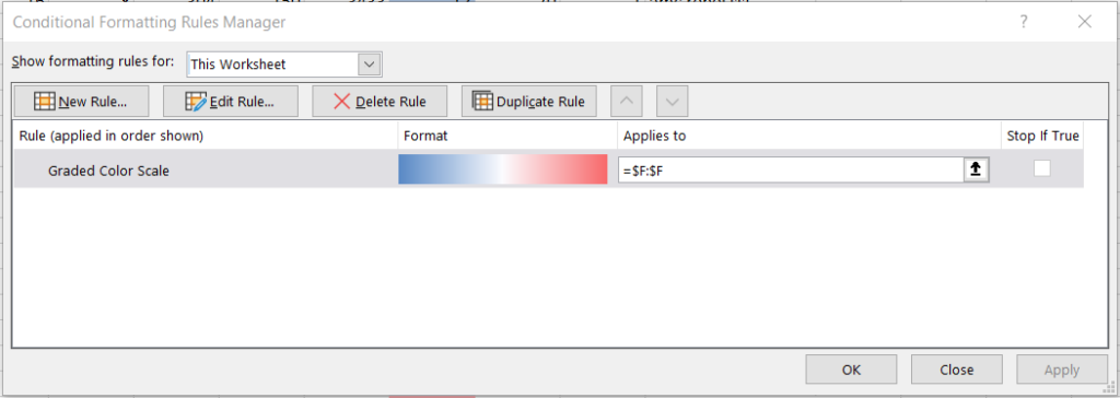
Selecting this option brings up a window that can be used to adjust the functionality of the rules you’ve already created:
Figure 7
First, next to the “Show formatting rules for” header, you can choose whether to display the already-created rules for the currently selected cells or for the entire worksheet.
There are six buttons on this window’s header: New Rule, Edit Rule, Delete Rule, Duplicate Rule, Move Up, and Move Down. New Rule brings up the same window we explored in the New Rule section. Edit Rule also brings up this same window, but with the selected existing rule already pre-populated; to use this button, first select a rule in the bottom section of the window, and then click Edit Rule. Delete Rule and Duplicate Rule are self-explanatory. Finally, Move Up and Move Down are used to alter the prioritization the rules you’ve created; you may have noticed that the leftmost column of the bottom section of the window is titled “Rule (applied in order shown)” and this is because it’s showing you the prioritization order of all created rules in the event that more than one rule applies to the same cell.
Lastly, we have the bottom section of the window, which shows each rule that’s been created, each rule’s format, the range of cells each rule applies to, and the Stop If True button, which if selected ensures that rules that fall below it won’t be executed if the former rule’s condition(s) is/are satisfied.
Whenever you make an alteration using the Manage Rules option, always click the Apply button in the lower right-hand corner before closing the window.
This blog post has been a very in-depth look into conditional formatting in Excel (most of what’s been covered is also available in Google Sheets). If you’re struggling to implement Conditional Formatting or any other features of Excel or another BI program at your workplace, contact us.