Interpreting Linear Regression Results
Interpreting Linear Regression Results
by Boxplot Apr 1, 2023
A Brief Introduction To Linear Regression
Linear regressions discover relationships between multiple variables by estimating a line or other function of best fit to a set of data. For example, the orange line is what a linear regression’s result would look like for the data shown in blue:
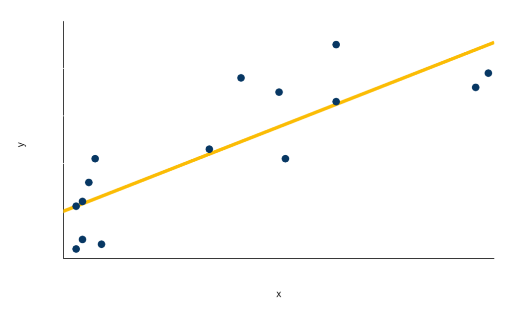
This function of best fit (shown here in orange) is expressed in the format of y = mx + b, where y is the variable we are trying to predict and x, sometimes referred to as a regressor, is the variable whose effect on y we are examining. Since m represents the slope of the line, it can be thought of as the effect of x on y (mathematically, m tells us the amount we would expect y to increase by for an increase of 1 in x, so m essentially tells us by how much x is affecting y). Thus, the orange line represents our best estimate of the relationship between x and y. Note two things. First, we can use linear regression to discover relationships between more than two variables; we are not limited to just one x variable to explain the y. Second, the relationship we estimate does not have to be a straight line as it is in this example; it can also be a polynomial function, an exponential function, etc.
Interpreting Linear Regression Results In Excel

I can see that the equation it gives for the best fit linear trend line is y = -0.0014x + 19.606. The main insight embedded in this equation is the -0.0014, which represents m from the previous section; this number tells us that every one-pound increase in the weight of a car results in a reduction of acceleration by 0.0014; a negative m means that an increase in the x variable is associated with a reduction in y and vice versa. Additionally, since our relationship is linear, we know that this relationship scales as well (so, for example, this value for m also tells us that every ten-pound increase in the weight of a car results in a reduction of acceleration by 0.014, every one-hundred-pound increase in the weight of a car results in a reduction of acceleration by 0.14, and so on).
In some cases, the intercept value b (19.606 in this case) is meaningful, but in this case, it is not. The intercept value tells us what we should expect the value of y to be if the value of x is 0. In this case, the value of x being 0 would translate to a car that weighs 0 pounds, which is obviously not meaningful.
So we’ve established that acceleration decreases by 0.0014 for every one-pound increase, but to understand the full influence of weight on acceleration, we also want to know: how much of the total variability in acceleration does weight account for? This is the question that a special metric called R2 answers. It’s called R2 because it’s the squared value of the correlation, which is represented by R. To get the R2 score on an Excel regression, go back into the formatting options that we used to add the regression equation, and check off the box for Display R2:
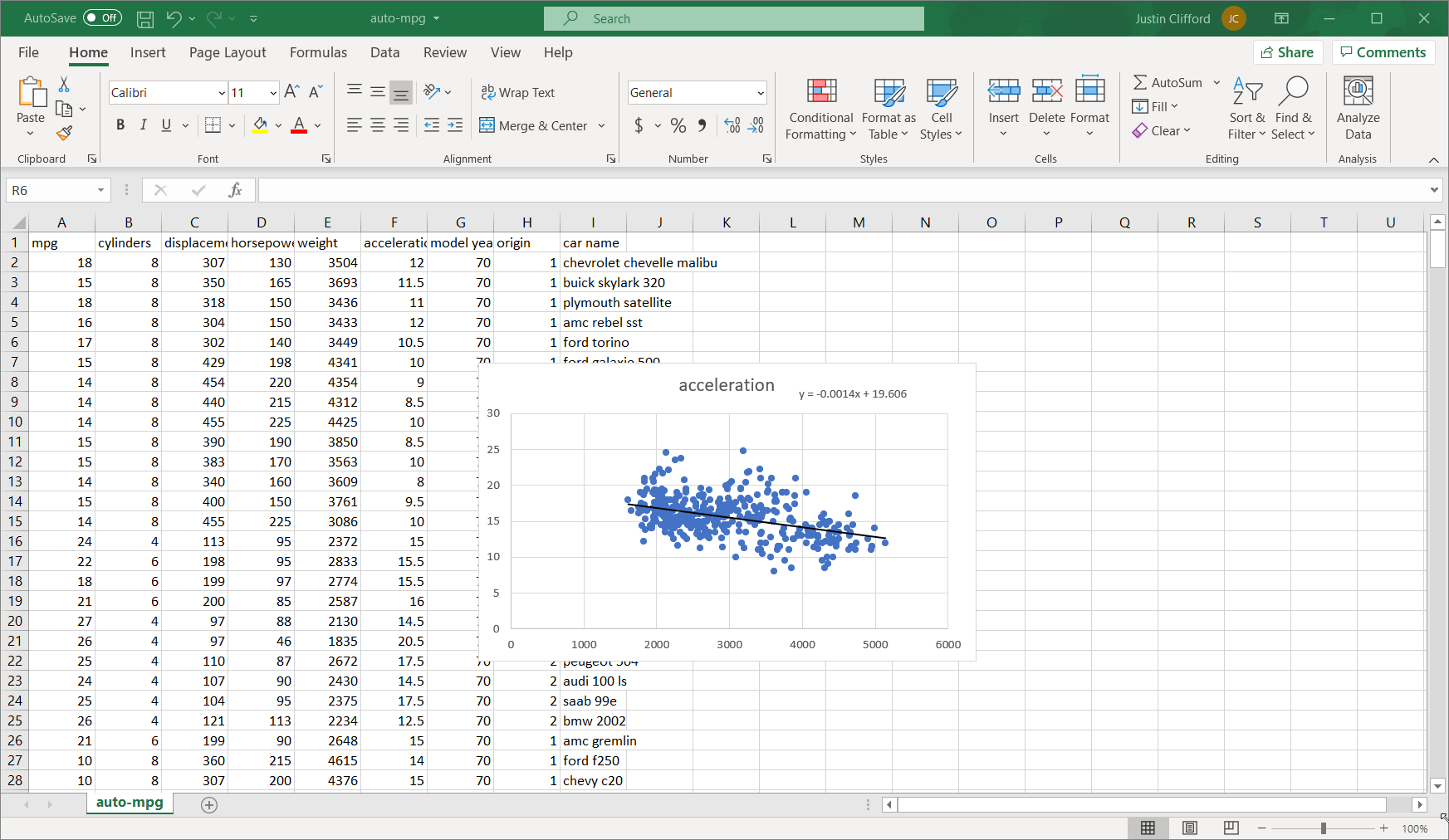
The resulting R2 value is 0.1743, which means that an estimated 17.43% of the variation in acceleration can be explained by weight.
Note that while it is possible to include more than one x variable in our regression to understand the effect of multiple variables on our chosen y, it is much better practice to use a programmatic tool such as R or Python rather than Excel for such cases.
Interpreting Linear Regression Results In Python And Other Programmatic Tools
Fire up your preferred Python IDE and load in the .csv or .xlsx file using the following code:

Obviously, you’ll have to replace the file path inside the read_csv method call with whatever file path and file name you saved the data under. There are two ways to run a linear regression in Python: by using the sklearn package and by using the statsmodels package. Here’s how to use Python’s sklearn package to run the regression (there are of course other ways of doing this, but this blog post is about interpreting results, not the actual coding):

Next, use reg’s coef_ attribute to retrieve the value of m:

Once again, we have arrived at a value of about -0.0014 for m. We can also check on the R2 value by using the score() method within reg:

and sure enough, it’s about 0.1743 again.
If we want to use the statsmodels package, the code to be run is:

The summary() method returns us a clean table which confirms the coefficient value of -0.0014, a constant (intercept) value of 19.606, and an R2 value of 0.1743:
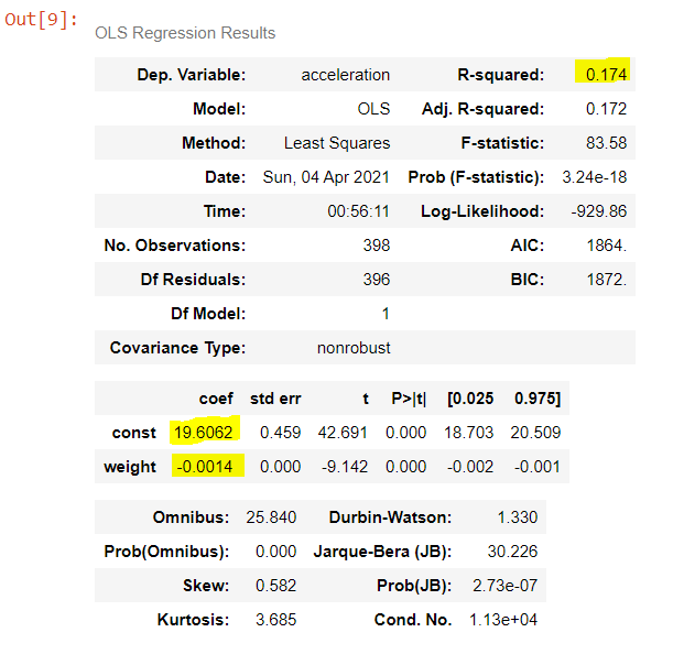
This table also gives us a bunch of other information. We won’t go through all of it in this blog post, but here are a few highlights:
- Adjusted R2: Tells us the R2 value adjusted for the number of regressors in the regression. It increases over regular R2 if new regressors improve R2 by an abnormally large amount. Since there is only one regressor in this regression, adjusted R2 is slightly lower than regular R2.
- Model: The Model is denoted as OLS, which stands for ordinary least squares. This is the standard form of linear regression that we’ve explored in this blog post.
- Df Model: Tells us the number of degrees of freedom in the model, which is the number of regressors in the regression.
- std err, t, and P>|t|: These metrics show which results are statistically significant, and which are not. Values in the std err column tell us the accuracy of the coef values, where lower std err values correspond to higher accuracy. Values in the t column tell us the t-values of the coef values, which indicates the number of standard errors away from 0 the coef values are. The t-values are very important ―especially in the row(s) that correspond to regressor(s)― because if a t-value is at or near 0, it means that the constant/regressor in that row has an effect of 0 on the y variable (i.e., the regressor is meaningless). But if a t-score is higher than about 2, it means that the regressor in that row is statistically significant. Finally, values in the P>|t| tell us the probability that the constant/regressor in that row is not equal to 0; if the P>|t| is high enough, we can therefore conclude that the constant/regressor is “significant”, i.e., we can be sure that that constant/regressor has a meaningful effect on the y variable.
While the exact command/syntax used for linear regressions varies among Python, R, SPSS, Stata, and other tools, each tool is able to give you similar information to what we looked at in Python and Excel.
<< Previous Post
"How B2C Businesses Can Use Their Data"
Next Post >>
"Tips For Building Likert Surveys"